Author: Maciej Nasinski
Check the miceFast website for more details
![]()
![]()
Overview
miceFast provides fast methods for imputing missing data, leveraging an object-oriented programming paradigm and optimized linear algebra routines.
The package includes convenient helper functions compatible with data.table, dplyr, and other popular R packages.
Major speed improvements occur when:
- Using a grouping variable, where the data is automatically sorted by group, significantly reducing computation time. - Performing multiple imputations, by evaluating the underlying quantitative model only once for multiple draws. - Running Predictive Mean Matching (PMM), thanks to presorting and binary search.
For performance details, see performance_validity.R in the extdata folder.
Vignettes:
Practical Advice
-
Only need a filled-in dataset for exploration or ML? A single imputation with
fill_NA()or averaging draws withfill_NA_N()is fast and convenient. For any inferential statement use full MI withpool(). -
Little missing data + MCAR? Consider using
complete.cases(). Listwise deletion is unbiased under MCAR and may be sufficient when the fraction of incomplete rows is small. -
For publication, always run a sensitivity analysis: compare MI results against base methods (
complete.cases(), mean imputation) and across different imputation models (lm_bayes,lm_noise,pmm). Vary the number of imputations. If conclusions change, investigate why. Report the imputation model, m, and any assumptions about the missing-data mechanism. - See the MI vignette for details on MCAR/MAR/MNAR mechanisms and a practical checklist.
Multiple Imputation Workflow
mice implements the full MI pipeline (impute, analyze, pool). miceFast focuses on the computationally expensive part: fitting the imputation models. It is typically ~10× faster than mice for the imputation step alone (see benchmarks). Two usage modes:
MI with Rubin’s rules. Call
fill_NA()with a stochastic model in a loop to create m completed datasets, thenpool()the fitted models. For continuous variables uselm_bayes(strictly proper; it draws from the posterior). For both continuous and categorical variables,pmm(Predictive Mean Matching) is also proper. It draws from the posterior and matches to observed values, preserving the data distribution. Use the OOP interface (impute("pmm", ...)) in a loop for MI with PMM. For categorical variables,ldawith a randomridgeis approximate (ad-hoc perturbation, not a posterior draw, but works well in practice).lm_noiseis improper (no parameter uncertainty); useful for sensitivity checks. See the MI vignette.Single-dataset imputation.
fill_NA_N()withlm_bayes/lm_noisereturns the mean of k stochastic draws per missing value. Withpmm, k is the number of nearest neighbours to sample from (no averaging). Handy for exploration, but not for Rubin’s rules (between-imputation variance is lost).Iterative FCS (chained equations). When multiple variables have interlocking (non-monotone) missingness, you can cycle through variables in a loop, restoring and re-imputing each one — the same algorithm mice uses. With a monotone pattern a single pass suffices and FCS is unnecessary. See the Introduction vignette for details.
See the MI vignette for worked examples.
Installation
You can install miceFast from CRAN:
install.packages("miceFast")Or install the development version from GitHub:
# install.packages("devtools")
devtools::install_github("polkas/miceFast")
Quick Example
dplyr
library(miceFast)
library(dplyr)

data(air_miss)

# Visualize the NA structure
upset_NA(air_miss, 6)

# Select the 4 core variables for regression: Ozone ~ Solar.R + Wind + Temp
# Ozone has 37 NAs, Solar.R has 7 NAs, Wind and Temp are complete.
df <- air_miss[, c("Ozone", "Solar.R", "Wind", "Temp")]

# MI with Rubin's rules: impute m = 10 datasets, fit model, pool.
# Impute Solar.R first (predictors fully observed), then Ozone
# (can now use the freshly imputed Solar.R). This sequential order
# resolves joint missingness in a single pass.
set.seed(1234)
completed <- lapply(1:10, function(i) {
  df %>%
    mutate(Solar.R = fill_NA(., "lm_bayes", "Solar.R", c("Wind", "Temp"))) %>%
    mutate(Ozone   = fill_NA(., "lm_bayes", "Ozone",   c("Solar.R", "Wind", "Temp")))
})
fits <- lapply(completed, function(d) lm(Ozone ~ Solar.R + Wind + Temp, data = d))
pool(fits)
#> Pooled results from 10 imputed datasets
#> Rubin's rules with Barnard-Rubin df adjustment
#>
#>         term  estimate std.error statistic    df   p.value
#>  (Intercept) -49.50313  21.74948    -2.276 78.41 2.557e-02
#>      Solar.R   0.05771   0.02294     2.516 72.83 1.407e-02
#>         Wind  -3.44033   0.62721    -5.485 76.15 5.185e-07
#>         Temp   1.47603   0.23404     6.307 97.50 8.345e-09
data.table
library(miceFast)
library(data.table)

data(air_miss)
dt <- as.data.table(air_miss[, c("Ozone", "Solar.R", "Wind", "Temp")])

# MI with Rubin's rules: same sequential chain as above.
set.seed(1234)
completed <- lapply(1:10, function(i) {
  d <- copy(dt)
  d[, Solar.R := fill_NA(.SD, "lm_bayes", "Solar.R", c("Wind", "Temp"))]
  d[, Ozone   := fill_NA(.SD, "lm_bayes", "Ozone",   c("Solar.R", "Wind", "Temp"))]
  d
})
fits <- lapply(completed, function(d) lm(Ozone ~ Solar.R + Wind + Temp, data = d))
pool(fits)
For iterative FCS (chained equations) with non-monotone missingness, see the Introduction vignette.
Naive imputation (baseline only)
# Quick baseline. Biased; does not account for relationships between variables.
naive_fill_NA(air_miss)
See the Introduction vignette for weights, the OOP interface, log-transformations, and more.
Key Features
-
Object-Oriented Interface via
miceFastobjects (Rcpp modules). -
Convenient Helpers:
-
fill_NA(): Single imputation (lda,lm_pred,lm_bayes,lm_noise).
-
fill_NA_N(): Multiple imputations. Averaged draws forlm_bayes/lm_noise; nearest-neighbour sampling forpmm.
-
pool(): Pool multiply imputed results using Rubin’s rules.
-
VIF(): Variance Inflation Factor calculations.
-
naive_fill_NA(): Automatic naive imputations.
-
compare_imp(): Compare original vs. imputed values.
-
upset_NA(): Visualize NA structure using UpSetR.
-
Quick Reference Table:
| Function | Description |
|---|---|
new(miceFast) |
Creates an OOP instance with numerous imputation methods (see the vignette). |
fill_NA() |
Single imputation: lda, lm_pred, lm_bayes, lm_noise. |
fill_NA_N() |
lm_bayes/lm_noise: averages k draws. pmm: samples from k nearest observed values (works for both continuous and categorical). |
pool() |
Pools estimates from m imputed datasets using Rubin’s rules. Works with any model that has coef() and vcov(). |
VIF() |
Computes Variance Inflation Factors. |
naive_fill_NA() |
Performs automatic, naive imputations. |
compare_imp() |
Compares imputations vs. original data. |
upset_NA() |
Visualizes NA structure using an UpSet plot. |
Performance Highlights
Median timings on 100k rows, 10 variables, 100 groups (R 4.4.3, macOS M3 Pro, optimized BLAS/LAPACK):
Imputation quality (SSE) is comparable to mice across all models.
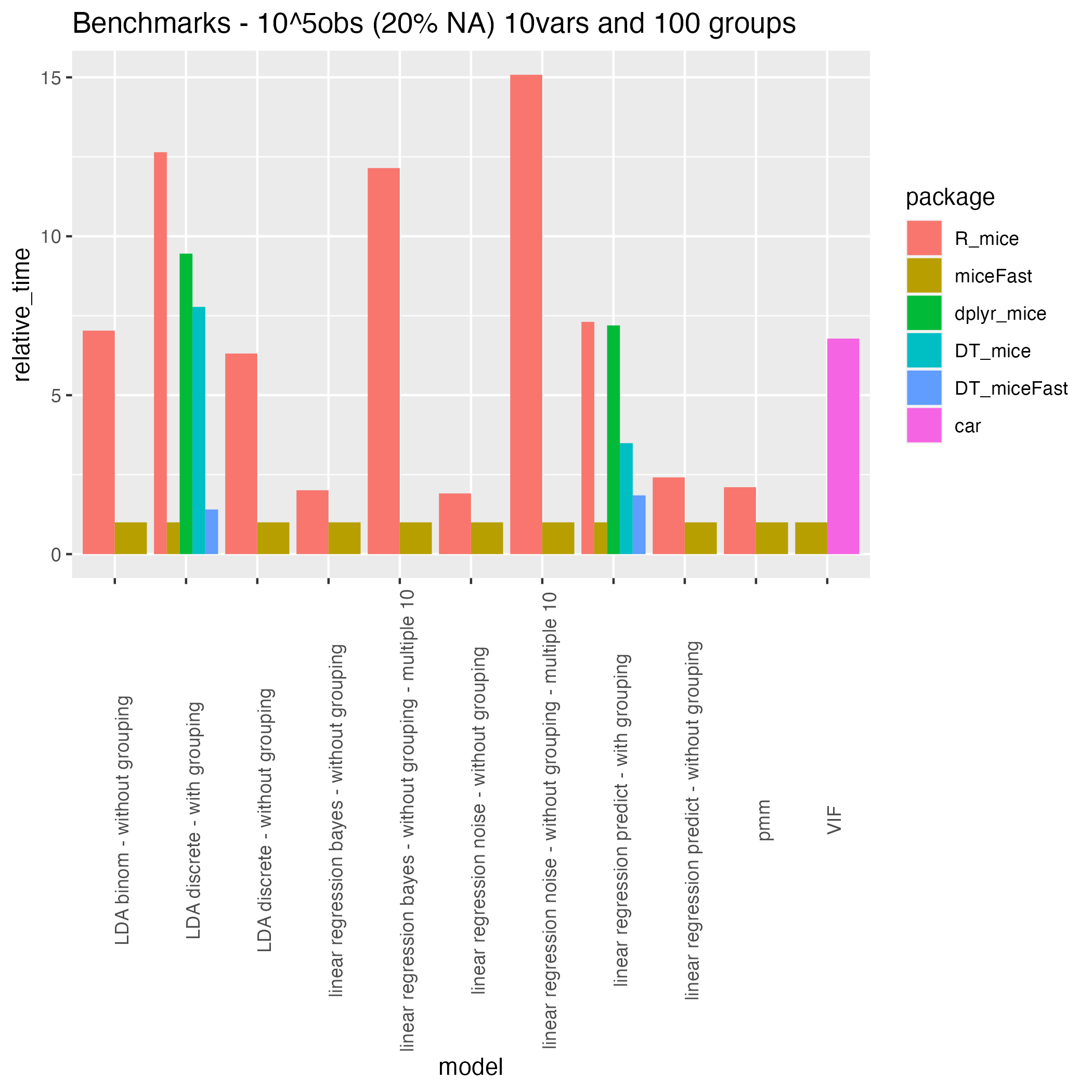
Full benchmark script: inst/extdata/performance_validity.R.