miceFast - Introduction and Advanced Usage • miceFast

Overview

miceFast provides fast imputation methods built on C++/RcppArmadillo (Eddelbuettel & Sanderson, 2014). The main interfaces are:

fill_NA and fill_NA_N — work with dplyr and data.table pipelines.
new(miceFast) — OOP interface for maximum control.
pool() — combine results from multiply imputed datasets using Rubin’s rules (Rubin, 1987) with the Barnard-Rubin (1999) degrees-of-freedom adjustment.

For missing-data theory (MCAR/MAR/MNAR) and full MI workflows, see the companion vignette: Missing Data Mechanisms and Multiple Imputation. For a comprehensive treatment, see van Buuren (2018).

library(miceFast)
library(dplyr)
library(data.table)
library(ggplot2)
set.seed(123456)

Available Imputation Models

miceFast supports several models via the model argument in fill_NA() and fill_NA_N():

Model	Type	Stochastic?	Use case
`lm_pred`	Linear regression	No	Deterministic point prediction. With only an `Intercept` column, equivalent to mean imputation.
`lm_bayes`	Bayesian linear regression	Yes	Draws coefficients from their posterior — recommended for MI of continuous variables.
`lm_noise`	Linear regression + noise	Yes	Adds residual noise to predictions — alternative stochastic model.
`lda`	Linear Discriminant Analysis	Conditional	For categorical variables. With a random `ridge` parameter it becomes stochastic, suitable for MI.
`pmm`	Predictive Mean Matching	Yes	Imputes from observed values via nearest-neighbor matching. Only available through `fill_NA_N()` / `impute_N()`.

For proper MI you need a stochastic model: lm_bayes or lm_noise for continuous variables, lda with ridge = runif(1, ...) for categorical.

Example Data

The package ships with air_miss, an extended version of airquality with additional columns including a character variable, weights, groups, and a categorized Ozone variable.

data(air_miss)
str(air_miss)

## 'data.frame':    153 obs. of  13 variables:
##  $ Ozone      : num  41 36 12 18 NA 28 23 19 8 NA ...
##  $ Solar.R    : num  190 118 149 313 NA NA 299 99 19 194 ...
##  $ Wind       : num  7.4 8 12.6 11.5 14.3 14.9 8.6 13.8 20.1 8.6 ...
##  $ Temp       : num  67 72 74 62 56 66 65 59 61 69 ...
##  $ Day        : num  1 2 3 4 5 6 7 8 9 10 ...
##  $ Intercept  : num  1 1 1 1 1 1 1 1 1 1 ...
##  $ index      : num  1 2 3 4 5 6 7 8 9 10 ...
##  $ weights    : num  1.019 1.011 0.989 0.991 0.995 ...
##  $ groups     : Factor w/ 5 levels "5","6","7","8",..: 1 1 1 1 1 1 1 1 1 1 ...
##  $ x_character: chr  "(140,210]" "(70,140]" "(140,210]" "(280,350]" ...
##  $ Ozone_chac : chr  "(40,60]" "(20,40]" "(0,20]" "(0,20]" ...
##  $ Ozone_f    : Factor w/ 8 levels "(0,20]","(20,40]",..: 3 2 1 1 NA 2 2 1 1 NA ...
##  $ Ozone_high : logi  FALSE FALSE FALSE FALSE NA FALSE ...

Examining Missingness

upset_NA(air_miss, 6)

Checking for Collinearity

Before imputing, check Variance Inflation Factors. Values above ~10 suggest problematic collinearity that can destabilize imputation models — consider dropping or combining redundant predictors before imputing.

VIF(
  air_miss,
  posit_y = "Ozone",
  posit_x = c("Solar.R", "Wind", "Temp", "x_character", "Day", "weights", "groups")
)

##           [,1]
## [1,] 24.978996
## [2,]  1.445308
## [3,]  3.077776
## [4,] 42.248792
## [5,]  1.083795
## [6,]  1.100853
## [7,]  2.954588

Single Imputation with `fill_NA()`

fill_NA() imputes missing values in a single column using a specified model and predictors. It accepts column names (strings) or position indices and works inside dplyr::mutate() or data.table := expressions.

Basic usage (dplyr)

data(air_miss)

result <- air_miss %>%
  # Continuous variable: Bayesian linear model (stochastic)
  mutate(Ozone_imp = fill_NA(
    x = .,
    model = "lm_bayes",
    posit_y = "Ozone",
    posit_x = c("Solar.R", "Wind", "Temp")
  )) %>%
  # Categorical variable: LDA
  mutate(x_char_imp = fill_NA(
    x = .,
    model = "lda",
    posit_y = "x_character",
    posit_x = c("Wind", "Temp")
  ))

head(result[, c("Ozone", "Ozone_imp", "x_character", "x_char_imp")])

##   Ozone Ozone_imp x_character x_char_imp
## 1    41        41   (140,210]  (140,210]
## 2    36        36    (70,140]   (70,140]
## 3    12        12   (140,210]  (140,210]
## 4    18        18   (280,350]  (280,350]
## 5    NA        NA        <NA>     (0,70]
## 6    28        28        <NA>     (0,70]

With weights and grouped imputation

Grouping fits a separate model per group, which is useful when the relationship between variables varies across subpopulations. Weights allow for heteroscedasticity or survey designs.

data(air_miss)

result_grouped <- air_miss %>%
  group_by(groups) %>%
  do(mutate(.,
    Solar_R_imp = fill_NA(
      x = .,
      model = "lm_pred",
      posit_y = "Solar.R",
      posit_x = c("Wind", "Temp", "Intercept"),
      w = .[["weights"]]
    )
  )) %>%
  ungroup()

head(result_grouped[, c("Solar.R", "Solar_R_imp", "groups")])

## # A tibble: 6 × 3
##   Solar.R Solar_R_imp groups
##     <dbl>       <dbl> <fct> 
## 1     190        190  5     
## 2     118        118  5     
## 3     149        149  5     
## 4     313        313  5     
## 5      NA        103. 5     
## 6      NA        176. 5

Log-transformation

For right-skewed variables (like Ozone), use logreg = TRUE to impute on the log scale. The model fits on $\log(y)$ and back-transforms the predictions:

data(air_miss)

result_log <- air_miss %>%
  mutate(Ozone_imp = fill_NA(
    x = .,
    model = "lm_bayes",
    posit_y = "Ozone",
    posit_x = c("Solar.R", "Wind", "Temp", "Intercept"),
    logreg = TRUE
  ))

# Compare distributions: log imputation avoids negative values
summary(result_log[c("Ozone", "Ozone_imp")])

##      Ozone          Ozone_imp     
##  Min.   :  1.00   Min.   :  1.00  
##  1st Qu.: 18.00   1st Qu.: 18.55  
##  Median : 31.50   Median : 30.00  
##  Mean   : 42.13   Mean   : 41.12  
##  3rd Qu.: 63.25   3rd Qu.: 59.00  
##  Max.   :168.00   Max.   :168.00  
##  NA's   :37       NA's   :2

Using column position indices

You can refer to columns by position instead of name. Check names(air_miss) to find the right positions:

data(air_miss)

result_pos <- air_miss %>%
  mutate(Ozone_imp = fill_NA(
    x = .,
    model = "lm_bayes",
    posit_y = 1,
    posit_x = c(4, 6),
    logreg = TRUE
  ))

head(result_pos[, c("Ozone", "Ozone_imp")])

##   Ozone Ozone_imp
## 1    41 41.000000
## 2    36 36.000000
## 3    12 12.000000
## 4    18 18.000000
## 5    NA  4.793808
## 6    28 28.000000

## Basic usage (data.table)

data(air_miss)
setDT(air_miss)

air_miss[, Ozone_imp := fill_NA(
  x = .SD,
  model = "lm_bayes",
  posit_y = "Ozone",
  posit_x = c("Solar.R", "Wind", "Temp")
)]

air_miss[, x_char_imp := fill_NA(
  x = .SD,
  model = "lda",
  posit_y = "x_character",
  posit_x = c("Wind", "Temp")
)]

# With grouping
air_miss[, Solar_R_imp := fill_NA(
  x = .SD,
  model = "lm_pred",
  posit_y = "Solar.R",
  posit_x = c("Wind", "Temp", "Intercept"),
  w = .SD[["weights"]]
), by = .(groups)]

Averaged Multiple Imputation with `fill_NA_N()`

fill_NA_N() generates k imputed values per missing observation and returns their average. This is useful for exploratory analysis or ML pipelines, but between-imputation variance is lost so Rubin’s rules cannot be applied. For inference, use the MI workflow with fill_NA() + pool() instead.

dplyr

data(air_miss)

result_n <- air_miss %>%
  # PMM with 20 draws — imputes from observed values
  mutate(Ozone_pmm = fill_NA_N(
    x = .,
    model = "pmm",
    posit_y = "Ozone",
    posit_x = c("Solar.R", "Wind", "Temp"),
    k = 20
  )) %>%
  # lm_noise with 30 draws and weights
  mutate(Ozone_noise = fill_NA_N(
    x = .,
    model = "lm_noise",
    posit_y = "Ozone",
    posit_x = c("Solar.R", "Wind", "Temp"),
    w = .[["weights"]],
    logreg = TRUE,
    k = 30
  ))

data.table with grouping

data(air_miss)
setDT(air_miss)

air_miss[, Ozone_pmm := fill_NA_N(
  x = .SD,
  model = "pmm",
  posit_y = "Ozone",
  posit_x = c("Wind", "Temp", "Intercept"),
  w = .SD[["weights"]],
  logreg = TRUE,
  k = 20
), by = .(groups)]

Comparing Imputations

Use compare_imp() to visually compare the distribution of observed vs. imputed values:

data(air_miss)

air_miss_imp <- air_miss %>%
  mutate(
    Ozone_bayes = fill_NA(x = ., model = "lm_bayes",
      posit_y = "Ozone", posit_x = c("Solar.R", "Wind", "Temp")),
    Ozone_pmm = fill_NA_N(x = ., model = "pmm",
      posit_y = "Ozone", posit_x = c("Solar.R", "Wind", "Temp"), k = 20)
  )

compare_imp(air_miss_imp, origin = "Ozone", target = c("Ozone_bayes", "Ozone_pmm"))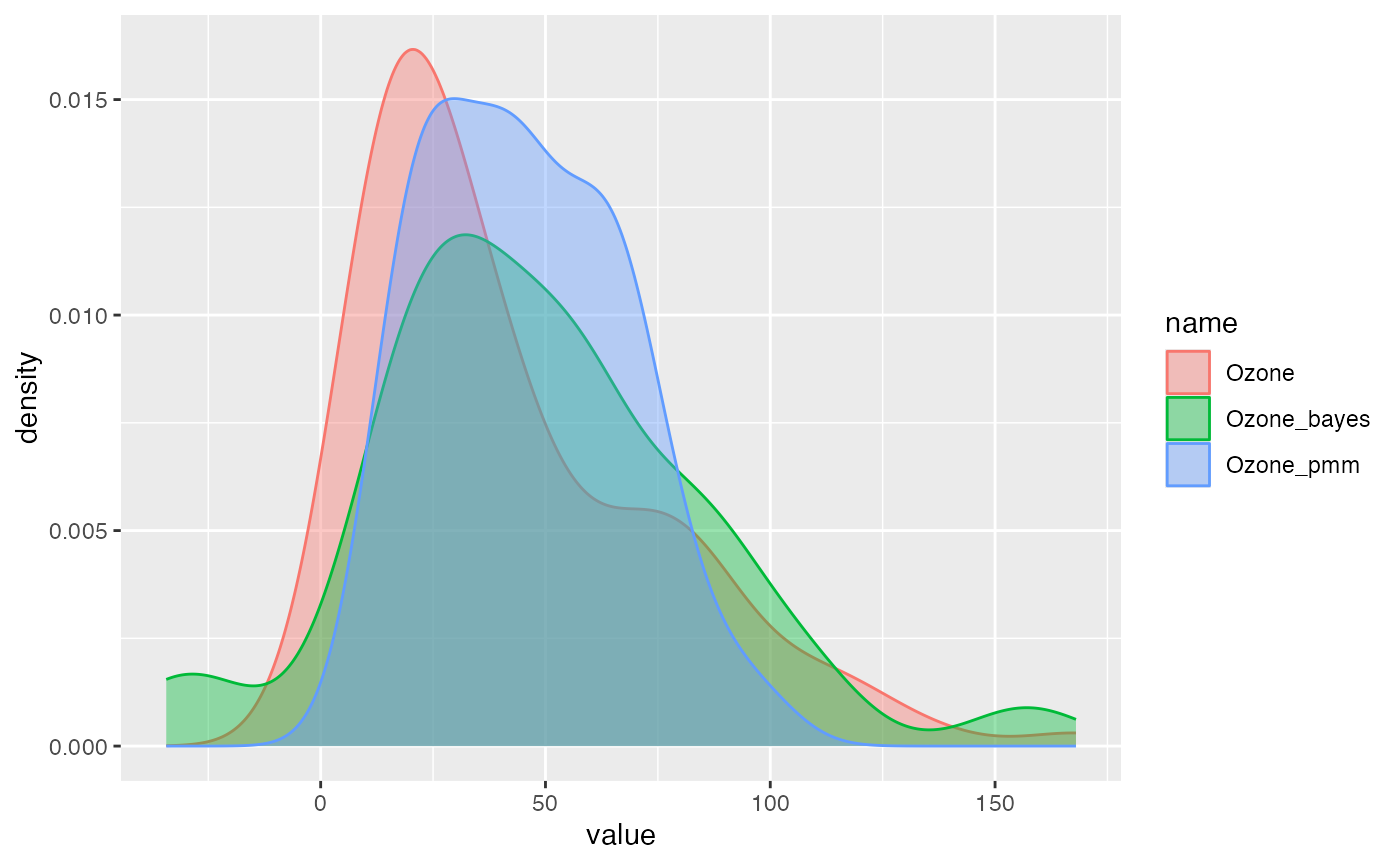

Multiple Imputation with `pool()`

For proper statistical inference on incomplete data, use the MI workflow:

Generate m completed datasets (each with a different stochastic imputation).
Fit your analysis model on each completed dataset.
Pool results using Rubin’s rules via pool().

pool() works with any model that has coef() and vcov() methods.

data(air_miss)

# Step 1: Generate m = 5 completed datasets
completed <- lapply(1:5, function(i) {
  air_miss %>%
    mutate(
      Ozone_imp = fill_NA(
        x = ., model = "lm_bayes",
        posit_y = "Ozone", posit_x = c("Solar.R", "Wind", "Temp")
      )
    )
})

# Step 2: Fit a model on each
fits <- lapply(completed, function(d) lm(Ozone_imp ~ Wind + Temp, data = d))

# Step 3: Pool using Rubin's rules
pool_res <- pool(fits)
pool_res

## Pooled results from 5 imputed datasets
## Rubin's rules with Barnard-Rubin df adjustment
## 
##         term estimate std.error statistic    df   p.value
##  (Intercept)  -62.880   25.4366    -2.472 29.24 1.949e-02
##         Wind   -3.378    0.7308    -4.622 24.29 1.057e-04
##         Temp    1.774    0.2575     6.889 44.98 1.491e-08

summary(pool_res)

## Pooled results from 5 imputed datasets
## Rubin's rules with Barnard-Rubin df adjustment
## Complete-data df: 148 
## 
## Coefficients:
##         term estimate std.error statistic    df   p.value conf.low conf.high
##  (Intercept)  -62.880   25.4366    -2.472 29.24 1.949e-02 -114.886   -10.875
##         Wind   -3.378    0.7308    -4.622 24.29 1.057e-04   -4.885    -1.870
##         Temp    1.774    0.2575     6.889 44.98 1.491e-08    1.255     2.292
## 
## Pooling diagnostics:
##         term      ubar         b         t    riv lambda    fmi
##  (Intercept) 445.46980 167.95979 647.02154 0.4524 0.3115 0.3542
##         Wind   0.34710   0.15578   0.53404 0.5386 0.3500 0.3977
##         Temp   0.05098   0.01276   0.06628 0.3003 0.2309 0.2630

Full Imputation: Filling All Variables and MI with Rubin’s Rules

In practice you often need to impute every variable that has missing values, then run MI with proper pooling. Below is a complete workflow using air_miss.

data(air_miss)

# Define a function that fills all variables with NAs in one pass
impute_all <- function(data) {
  data %>%
    # Continuous: Ozone (log-normal, use logreg)
    mutate(Ozone_imp = fill_NA(
      x = ., model = "lm_bayes",
      posit_y = "Ozone",
      posit_x = c("Solar.R", "Wind", "Temp"),
      logreg = TRUE
    )) %>%
    # Continuous: Solar.R
    mutate(Solar_R_imp = fill_NA(
      x = ., model = "lm_bayes",
      posit_y = "Solar.R",
      posit_x = c("Wind", "Temp", "Intercept"),
      w = weights
    )) %>%
    # Categorical: x_character (LDA with random ridge for stochasticity)
    mutate(x_char_imp = fill_NA(
      x = ., model = "lda",
      posit_y = "x_character",
      posit_x = c("Wind", "Temp"),
      ridge = runif(1, 0.5, 50)
    )) %>%
    # Categorical: Ozone_chac (use tryCatch for safety with small groups)
    group_by(groups) %>%
    do(mutate(., Ozone_chac_imp = tryCatch(
      fill_NA(
        x = ., model = "lda",
        posit_y = "Ozone_chac",
        posit_x = c("Temp", "Wind")
      ),
      error = function(e) .[["Ozone_chac"]]
    ))) %>%
    ungroup()
}

# MI: generate m = 10 completed datasets
set.seed(2024)
m <- 10
completed <- lapply(1:m, function(i) impute_all(air_miss))

# Fit the analysis model on each completed dataset
fits <- lapply(completed, function(d) lm(Ozone_imp ~ Wind + Temp + Solar_R_imp, data = d))

# Pool using Rubin's rules
pool_result <- pool(fits)
pool_result

## Pooled results from 10 imputed datasets
## Rubin's rules with Barnard-Rubin df adjustment
## 
##         term  estimate std.error statistic    df   p.value
##  (Intercept) -84.34373  25.81112    -3.268 47.70 2.014e-03
##         Wind  -2.53190   0.67967    -3.725 68.08 3.986e-04
##         Temp   1.77575   0.28604     6.208 47.86 1.218e-07
##  Solar_R_imp   0.07218   0.02492     2.897 59.38 5.275e-03

summary(pool_result)

## Pooled results from 10 imputed datasets
## Rubin's rules with Barnard-Rubin df adjustment
## Complete-data df: 147 
## 
## Coefficients:
##         term  estimate std.error statistic    df   p.value   conf.low conf.high
##  (Intercept) -84.34373  25.81112    -3.268 47.70 2.014e-03 -136.24880   -32.439
##         Wind  -2.53190   0.67967    -3.725 68.08 3.986e-04   -3.88814    -1.176
##         Temp   1.77575   0.28604     6.208 47.86 1.218e-07    1.20059     2.351
##  Solar_R_imp   0.07218   0.02492     2.897 59.38 5.275e-03    0.02232     0.122
## 
## Pooling diagnostics:
##         term      ubar         b         t    riv lambda    fmi
##  (Intercept) 4.574e+02 1.899e+02 6.662e+02 0.4566 0.3135 0.3406
##         Wind 3.568e-01 9.562e-02 4.620e-01 0.2948 0.2277 0.2494
##         Temp 5.623e-02 2.326e-02 8.182e-02 0.4549 0.3127 0.3397
##  Solar_R_imp 4.595e-04 1.469e-04 6.210e-04 0.3517 0.2602 0.2839

The same workflow using data.table:

data(air_miss)
setDT(air_miss)

impute_all_dt <- function(dt) {
  d <- copy(dt)
  d[, Ozone_imp := fill_NA(
    x = .SD, model = "lm_bayes",
    posit_y = "Ozone", posit_x = c("Solar.R", "Wind", "Temp"),
    logreg = TRUE
  )]
  d[, Solar_R_imp := fill_NA(
    x = .SD, model = "lm_bayes",
    posit_y = "Solar.R",
    posit_x = c("Wind", "Temp", "Intercept"),
    w = .SD[["weights"]]
  )]
  d[, x_char_imp := fill_NA(
    x = .SD, model = "lda",
    posit_y = "x_character", posit_x = c("Wind", "Temp"),
    ridge = runif(1, 0.5, 50)
  )]
  d[, Ozone_chac_imp := tryCatch(
    fill_NA(
      x = .SD, model = "lda",
      posit_y = "Ozone_chac", posit_x = c("Temp", "Wind")
    ),
    error = function(e) .SD[["Ozone_chac"]]
  ), by = .(groups)]
  d
}

set.seed(2024)
completed_dt <- lapply(1:10, function(i) impute_all_dt(air_miss))
fits_dt <- lapply(completed_dt, function(d) lm(Ozone_imp ~ Wind + Temp + Solar_R_imp, data = d))
pool(fits_dt)

## Pooled results from 10 imputed datasets
## Rubin's rules with Barnard-Rubin df adjustment
## 
##         term  estimate std.error statistic    df   p.value
##  (Intercept) -84.34373  25.81112    -3.268 47.70 2.014e-03
##         Wind  -2.53190   0.67967    -3.725 68.08 3.986e-04
##         Temp   1.77575   0.28604     6.208 47.86 1.218e-07
##  Solar_R_imp   0.07218   0.02492     2.897 59.38 5.275e-03

The `miceFast` OOP Module

For maximum performance and fine-grained control, use the C++ object directly. This interface operates on numeric matrices and uses column position indices.

Methods

Method	Description
`set_data(x)`	Set the data matrix (by reference).
`set_g(g)`	Set a grouping variable (positive numeric, no NAs).
`set_w(w)`	Set a weighting variable (positive numeric, no NAs).
`impute(model, y, x)`	Single imputation.
`impute_N(model, y, x, k)`	Averaged multiple imputation (k draws).
`update_var(y, imps)`	Permanently update a column with imputations.
`vifs(y, x)`	Variance Inflation Factors.
`get_data()` / `get_g()` / `get_w()` / `get_index()`	Retrieve data or metadata.
`sort_byg()` / `is_sorted_byg()`	Sort by grouping variable.
`which_updated()`	Check which columns have been updated.

Note that update_var() permanently alters the data matrix by reference. When a grouping variable is set, data is automatically sorted on first imputation; use get_index() to recover the original row order.

Simple example

data <- cbind(as.matrix(airquality[, 1:4]), intercept = 1, index = 1:nrow(airquality))
model <- new(miceFast)
model$set_data(data)

# Single imputation with linear model (col 1 = Ozone)
model$update_var(1, model$impute("lm_pred", 1, 5)$imputations)

# Averaged multiple imputation for Solar.R (col 2, Bayesian, k=10 draws)
model$update_var(2, model$impute_N("lm_bayes", 2, c(1, 3, 4, 5), k = 10)$imputations)

model$which_updated()

## [1] 1 2

head(model$get_data(), 4)

##      [,1] [,2] [,3] [,4] [,5] [,6]
## [1,]   41  190  7.4   67    1    1
## [2,]   36  118  8.0   72    1    2
## [3,]   12  149 12.6   74    1    3
## [4,]   18  313 11.5   62    1    4

With weights and groups

data <- cbind(as.matrix(airquality[, -5]), intercept = 1, index = 1:nrow(airquality))
weights <- rgamma(nrow(data), 3, 3)
groups <- as.numeric(airquality[, 5])

model <- new(miceFast)
model$set_data(data)
model$set_w(weights)
model$set_g(groups)

model$update_var(1, model$impute("lm_pred", 1, 6)$imputations)
model$update_var(2, model$impute_N("lm_bayes", 2, c(1, 3, 4, 5, 6), k = 10)$imputations)

# Recover original row order
head(cbind(model$get_data(), model$get_g(), model$get_w())[order(model$get_index()), ], 4)

##      [,1] [,2] [,3] [,4] [,5] [,6] [,7] [,8]      [,9]
## [1,]   41  190  7.4   67    1    1    1    5 0.8231504
## [2,]   36  118  8.0   72    2    1    2    5 0.4484750
## [3,]   12  149 12.6   74    3    1    3    5 1.2809177
## [4,]   18  313 11.5   62    4    1    4    5 0.8794161

With unsorted groups

When groups are not pre-sorted, the data is automatically sorted on first imputation:

data <- cbind(as.matrix(airquality[, -5]), intercept = 1, index = 1:nrow(airquality))
weights <- rgamma(nrow(data), 3, 3)
groups <- as.numeric(sample(1:8, nrow(data), replace = TRUE))

model <- new(miceFast)
model$set_data(data)
model$set_w(weights)
model$set_g(groups)

model$update_var(1, model$impute("lm_pred", 1, 6)$imputations)
model$update_var(2, model$impute_N("lm_bayes", 2, c(1, 3, 4, 5, 6), 10)$imputations)

head(cbind(model$get_data(), model$get_g(), model$get_w())[order(model$get_index()), ], 4)

##      [,1] [,2] [,3] [,4] [,5] [,6] [,7] [,8]      [,9]
## [1,]   41  190  7.4   67    1    1    1    2 0.9511796
## [2,]   36  118  8.0   72    2    1    2    3 0.4506585
## [3,]   12  149 12.6   74    3    1    3    6 0.7855931
## [4,]   18  313 11.5   62    4    1    4    3 0.7883065

Full MI workflow with OOP

The OOP interface can also drive the full MI loop. Each iteration creates a fresh model, imputes all variables with missing values, and returns the completed matrix in the original row order.

data(air_miss)

# Prepare a numeric matrix with an intercept and row index
mat <- cbind(
  as.matrix(air_miss[, c("Ozone", "Solar.R", "Wind", "Temp")]),
  intercept = 1,
  index = seq_len(nrow(air_miss))
)
groups <- as.numeric(air_miss$groups)

impute_oop <- function(mat, groups) {
  m <- new(miceFast)
  m$set_data(mat + 0)  # copy — set_data uses the matrix by reference
  m$set_g(groups)
  # col 1 = Ozone, col 2 = Solar.R, col 3 = Wind, col 4 = Temp, col 5 = intercept
  m$update_var(1, m$impute("lm_bayes", 1, c(2, 3, 4))$imputations)
  m$update_var(2, m$impute("lm_bayes", 2, c(3, 4, 5))$imputations)
  completed <- m$get_data()[order(m$get_index()), ]
  as.data.frame(completed)
}

set.seed(2025)
completed <- lapply(1:10, function(i) impute_oop(mat, groups))

fits <- lapply(completed, function(d) lm(V1 ~ V3 + V4, data = d))
pool(fits)

## Pooled results from 10 imputed datasets
## Rubin's rules with Barnard-Rubin df adjustment
## 
##         term estimate std.error statistic    df   p.value
##  (Intercept)  -69.010   25.8410    -2.671 62.19 9.651e-03
##           V3   -2.659    0.7687    -3.459 43.12 1.233e-03
##           V4    1.751    0.2681     6.530 76.01 6.646e-09

summary(pool(fits))

## Pooled results from 10 imputed datasets
## Rubin's rules with Barnard-Rubin df adjustment
## Complete-data df: 148 
## 
## Coefficients:
##         term estimate std.error statistic    df   p.value conf.low conf.high
##  (Intercept)  -69.010   25.8410    -2.671 62.19 9.651e-03 -120.663   -17.358
##           V3   -2.659    0.7687    -3.459 43.12 1.233e-03   -4.209    -1.109
##           V4    1.751    0.2681     6.530 76.01 6.646e-09    1.217     2.285
## 
## Pooling diagnostics:
##         term     ubar         b         t    riv lambda    fmi
##  (Intercept) 500.7617 151.81238 667.75527 0.3335 0.2501 0.2731
##           V3   0.3902   0.18250   0.59094 0.5145 0.3397 0.3684
##           V4   0.0573   0.01325   0.07188 0.2543 0.2028 0.2229

Generating Correlated Data with `corrData`

The corrData module generates correlated data for simulations. This is useful for creating test datasets with known properties.

# 3 continuous variables, 100 observations
means <- c(10, 20, 30)
cor_matrix <- matrix(c(
  1.0, 0.7, 0.3,
  0.7, 1.0, 0.5,
  0.3, 0.5, 1.0
), nrow = 3)

cd <- new(corrData, 100, means, cor_matrix)
sim_data <- cd$fill("contin")
round(cor(sim_data), 2)

##      [,1] [,2] [,3]
## [1,] 1.00 0.78 0.32
## [2,] 0.78 1.00 0.46
## [3,] 0.32 0.46 1.00

# With 2 categorical variables: first argument is nr_cat
cd2 <- new(corrData, 2, 200, means, cor_matrix)
sim_discrete <- cd2$fill("discrete")
head(sim_discrete)

##      [,1]     [,2]     [,3]
## [1,]    1 19.68768 29.40270
## [2,]    2 20.13020 28.32714
## [3,]    1 19.49938 30.97424
## [4,]    2 19.80052 30.02937
## [5,]    1 19.34898 29.39342
## [6,]    2 19.83346 29.67114

Tips

Creating matrices from data frames: R matrices hold only one type. Convert factors with model.matrix():
```
mtcars$cyl <- factor(mtcars$cyl)
model.matrix(~ ., data = mtcars, na.action = "na.pass")
```
Collinearity: Always check VIF() before imputing. High VIF (>10) indicates collinearity that can destabilize imputation models.

Error handling with groups: Small groups may not have enough observations. Wrap fill_NA() calls in tryCatch():

tryCatch(
  fill_NA(x = ., model = "lda", posit_y = "y", posit_x = c("x1", "x2")),
  error = function(e) .[["y"]]
)

BLAS optimization: Install an optimized BLAS library for significant speedups:
- Linux: sudo apt-get install libopenblas-dev
- macOS: See R macOS FAQ

References

Rubin, D.B. (1987). Multiple Imputation for Nonresponse in Surveys. John Wiley & Sons.
Barnard, J. and Rubin, D.B. (1999). Small-sample degrees of freedom with multiple imputation. Biometrika, 86(4), 948-955.
van Buuren, S. (2018). Flexible Imputation of Missing Data (2nd ed.). Chapman & Hall/CRC.
Eddelbuettel, D. and Sanderson, C. (2014). RcppArmadillo: Accelerating R with high-performance C++ linear algebra. Computational Statistics and Data Analysis, 71, 1054-1063.

miceFast - Introduction and Advanced Usage

Maciej Nasinski

2026-02-25

Overview

Available Imputation Models

Example Data

Examining Missingness

Checking for Collinearity

Single Imputation with `fill_NA()`

Basic usage (dplyr)

With weights and grouped imputation

Log-transformation

Using column position indices

Averaged Multiple Imputation with `fill_NA_N()`

dplyr

data.table with grouping

Comparing Imputations

Multiple Imputation with `pool()`

Full Imputation: Filling All Variables and MI with Rubin’s Rules

The `miceFast` OOP Module

Methods

Simple example

With weights and groups

With unsorted groups

Full MI workflow with OOP

Generating Correlated Data with `corrData`

Tips

References

miceFast - Introduction and Advanced Usage

Maciej Nasinski

2026-02-25

Overview

Available Imputation Models

Example Data

Examining Missingness

Checking for Collinearity

Single Imputation with fill_NA()

Basic usage (dplyr)

With weights and grouped imputation

Log-transformation

Using column position indices

Averaged Multiple Imputation with fill_NA_N()

dplyr

data.table with grouping

Comparing Imputations

Multiple Imputation with pool()

Full Imputation: Filling All Variables and MI with Rubin’s Rules

The miceFast OOP Module

Methods

Simple example

With weights and groups

With unsorted groups

Full MI workflow with OOP

Generating Correlated Data with corrData

Tips

References

Single Imputation with `fill_NA()`

Averaged Multiple Imputation with `fill_NA_N()`

Multiple Imputation with `pool()`

The `miceFast` OOP Module

Generating Correlated Data with `corrData`