Get Started with cat2cat

What is cat2cat?

cat2cat harmonizes categorical variables whose encoding changes over time - occupation codes (ISCO revisions), disease classifications (ICD-9 -> ICD-10), industry codes (NACE), product taxonomies.

Data type	Example	Function
Longitudinal data	Survey responses, administrative records	`cat2cat()`
(rotational) Panel data	Subjects observed in multiple periods	`cat2cat()` with `id_var`
Aggregated counts	Published statistics, summary tables	`cat2cat_agg()`

How to read the documentation

Use the package documentation in this order:

This vignette for the core problem, the main assumptions, and a minimal two-period workflow.
Choosing Weights and Validating ML when you need to decide between naive, frequency, and ML weights.
Advanced Workflows for multi-period chaining, (rotational) panels with id_var, aggregated data, and regression workflows.

If you only need a standard two-period harmonisation with default frequency weights, this vignette is usually enough.

The Problem

Classifications evolve. When they do, one old category maps to multiple new ones (and vice versa):

# Old occupation code "1111" became three different codes in the new system
trans[trans$old == "1111", ]
#>    old    new
#> 1 1111 111101
#> 2 1111 111102
#> 3 1111 111103

A worker coded 1111 in 2008 could be 111101, 111102, or 111103 in 2010. Which one? The original data doesn’t say.

Naive approaches fail:

Ignoring the problem leads to biased comparisons
Manual assignment is arbitrary and not reproducible

The Solution

cat2cat uses an approach:

The mapping table specifies how categories from one classification (e.g., the old one) correspond to categories from a second classification (e.g., the new one).
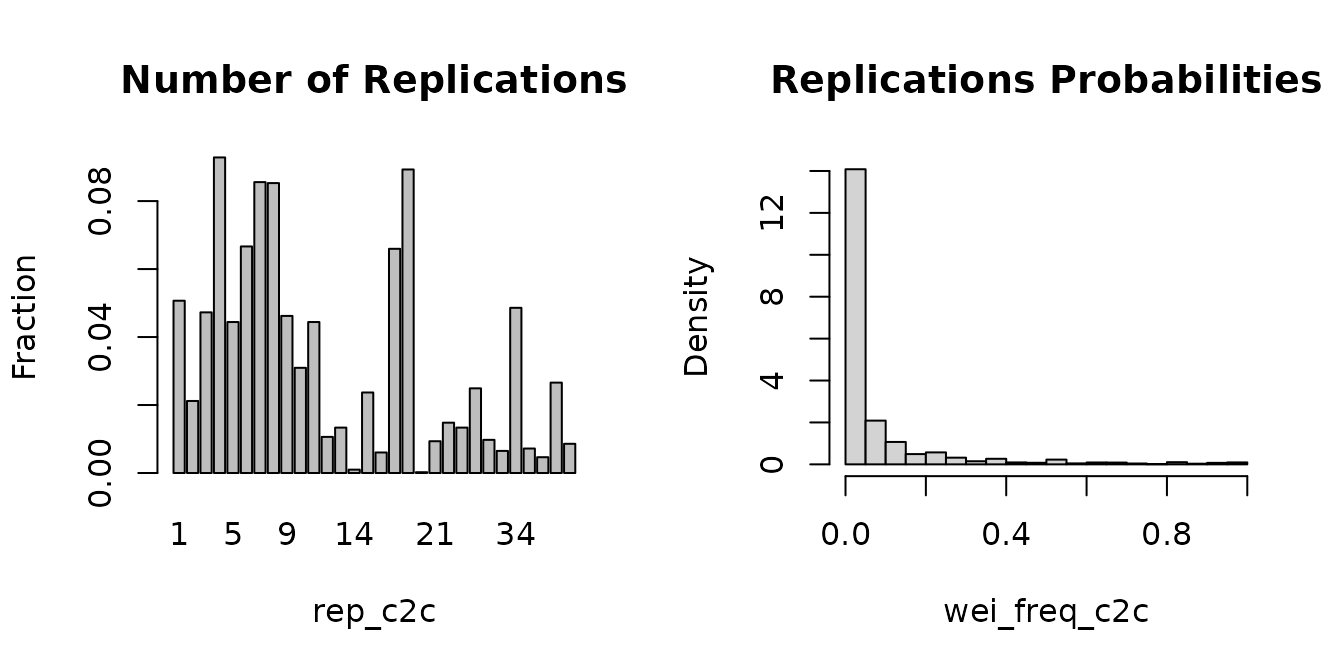
When one category corresponds to multiple categories in another system, the observation is replicated an equal number of times.
The replication probabilities (weights) sum to one and can be constructed using different rules.
The weights can be based on frequencies from the previous period, a uniform split, or ML algorithms.

Formally, for each original observation $i$ mapped to $k$ candidate categories, the weights satisfy:

$w_{ij} \geq 0 \quad \text{and} \quad \sum_{j=1}^{k} w_{ij} = 1$

This constraint ensures that replication is neutral for weighted statistics that do not use the unresolved mapped category.

For estimands that do not directly depend on the unresolved mapped category, the weighted point estimates are unchanged by replication. Inference still needs correction because replication increases the row count. See Nasinski et al. (2020) for the theoretical foundation and Nasinski & Gajowniczek (2023) for R implementation details.

Value Added of cat2cat

cat2cat separates true structural change from coding-system change. This is the main value for longitudinal analysis.

After harmonisation, you can:

Track trends within specific groups (for example occupations, industries, diagnoses) across waves
Compare subgroup dynamics on one consistent coding scheme
Estimate models with group-level effects and interactions without period-specific recoding artifacts
Run sensitivity checks across weighting assumptions and report uncertainty transparently

Without harmonisation, measured differences between periods can be driven by reclassification rules rather than real changes in the population.

Harmonisation Assumptions and Sensitivity

Suppose a worker is coded “1111” in 2008 and the mapping table says this code can correspond to “111101”, “111102”, or “111103” in 2010. The mapping table tells us the feasible target categories, but it does not tell us which target code this particular observation would have received under the 2010 classification.

This is the key assumption in probabilistic harmonisation. cat2cat does not discover the true latent split from the mapping table alone. Instead, it applies a transparent rule for distributing each ambiguous observation across its feasible target categories. Different rules can imply different weights while remaining consistent with the same observed data.

The workflow is therefore sequential. First, choose a harmonisation rule: naive, frequency, or ML. Conditional on that rule, cat2cat constructs the weights. Second, estimate the substantive quantity of interest - for example a mean, trend, group comparison, or OLS coefficient - on the harmonised data.

Identification is therefore a property of the estimate or model fitted after harmonisation, not of cat2cat alone. When the harmonised category enters that model, the chosen cat2cat rule becomes part of the model’s maintained assumptions.

The weighting rule matters only for observations with rep_c2c > 1. If a mapping is deterministic and no observation is replicated, the choice between naive, frequency, and ML weights is irrelevant. A deterministic recode still relies on the mapping table being correct, but it does not require a distributional assumption over candidate categories.

In anonymous repeated cross-sections, harmonisation is a counterfactual recoding exercise: it asks how an old code should be expressed in the target classification, not whether the same anonymous person kept the same occupation over time. In panel data with id_var, returning subjects are observed in both periods, so their categories can be linked directly rather than assigned probabilistically.

Sensitivity checks are most important when the final analysis uses the harmonised category itself, for example as a grouping variable, fixed effect, or interaction term. If results are similar under naive, frequency, and ML weights, conclusions are less dependent on the harmonisation assumption. If results differ, report the range and explain which assumption drives the difference. See Advanced Workflows for the model-level picture.

Three weighting schemes

Each weighting method adds one harmonisation assumption:

Naive weights (wei_naive_c2c): Assume a uniform distribution - each candidate is equally likely. $w_j = \frac{1}{k}$ This is the maximum entropy (least informative) prior. It requires only the mapping table - no data from either period. Use when you have no information favoring any candidate, or as a robustness bound.

Frequency weights (wei_freq_c2c): Assume that ambiguous observations are distributed as in the base-period population. $w_j = \frac{n_j^{\text{base}}}{\sum_{j'} n_{j'}^{\text{base}}}$ This requires observed counts in the base period. It works well when ambiguous cases resemble the overall population; it breaks down when they differ systematically (e.g., workers in transitional occupations may not match the stable population).

ML weights (wei_*_c2c for knn, rf, lda): Assume that individual features predict category membership. $w_j = P(j \mid X_i, g)$ This requires training data with both the category and predictive features. ML can correct for heterogeneity that frequency weights miss - if a 25-year-old programmer is more likely in “111101” than a 55-year-old manager, ML captures this. Use cat2cat_ml_run() to verify ML improves over baselines.

When each assumption matters

Method	Assumption fails when…	Practical check
Naive	Distribution is highly skewed	Compare `wei_naive_c2c` vs `wei_freq_c2c` - large differences suggest uniform is wrong
Frequency	Ambiguous cases differ from population	Compare ML vs freq accuracy in `cat2cat_ml_run()`
ML	Features don’t predict category	ML accuracy ≈ frequency accuracy in `cat2cat_ml_run()`

Reducing assumption dependence

The weighting assumption only affects observations that are replicated (rep_c2c > 1).

Strategies to reduce replication:

Panel id_var: returning subjects get direct matches - no replication. See Advanced Workflows.
Forward mapping: replicates the newer (more granular) period, which often maps 1-to-1 backward.
Code truncation: collapsing 6-digit to 4-digit codes often creates more 1-to-1 mappings in hierarchical systems (ISCO, ICD, NACE), especially for backward mapping. For forward mapping, truncation can also increase replication in some mappings.

If most observations have rep_c2c = 1, results depend minimally on the assumption.

Sensitivity check: run analyses with wei_naive_c2c, wei_freq_c2c, and ML weights. Similar conclusions -> robust. Divergent -> report the range.

When cat2cat won’t help

Blockers (cat2cat cannot be applied):

No mapping table: cat2cat requires a crosswalk. Alternative: expert coding or separate analyses per period.
Unobserved category: cat2cat harmonizes observed codes. Missing category is a missing-data problem - impute first.

Method-specific limits (workarounds exist):

Empty base categories: frequency weights fall back to naive (1/k). Use wei_naive_c2c or ML with external training data.
Few observations per ML class: models fail or overfit. Use frequency weights or coarser categories.

Naive weights (wei_naive_c2c) always work - they require only the mapping table.

Diagnostic:

check mean(rep_c2c) and cor(wei_freq_c2c, wei_naive_c2c). Very high replication or correlation near 1 suggests the mapping is too diffuse to improve over uniform weights. See Advanced Workflows for truncation strategies.

If you need something more advanced

This vignette focuses on the standard two-period micro-data workflow. Move to the other vignettes when:

you need to decide whether ML improves on simpler baselines,
you need to chain mappings across 3 or more waves,
you have a rotational panel with stable identifiers,
you only have aggregated counts rather than individual observations,
or your main task is regression and inference after harmonisation.

Use Cases

Repeated cross-sections (most common): harmonize independent surveys using base-period frequencies. The Quick Example below demonstrates this.

Multi-period analysis (3+ waves): chain cat2cat() calls sequentially - each step uses the previous step’s mapped frequencies. See Advanced Workflows.

Panel data (subjects observed in multiple periods): provide id_var to directly match returning subjects - no replication for them, only new entrants go through the probabilistic path. See Advanced Workflows.

If every subject is observed in both periods and the target-period category is known, cat2cat() may not be necessary: you can often join the target category back to the earlier record by id_var. cat2cat() is useful when some records cannot be linked directly and still need the mapping-table replication path.

Aggregated data (published counts only, no micro-data): use cat2cat_agg() with explicit equations:

library(dplyr)
data(verticals, package = "cat2cat")

agg_old <- verticals[verticals$v_date == "2020-04-01", ]
agg_new <- verticals[verticals$v_date == "2020-05-01", ]

agg_result <- cat2cat_agg(
  data = list(
    old = agg_old,
    new = agg_new,
    cat_var = "vertical",
    time_var = "v_date",
    freq_var = "counts"
  ),
  # Backward mapping: old Automotive split into Automotive1 + Automotive2
  Automotive %<% c(Automotive1, Automotive2),
  # Forward mapping: Kids1 + Kids2 merged into Kids  
  c(Kids1, Kids2) %>% c(Kids)
)

agg_result$old[c("vertical", "prop_c2c", "counts")]
#>        vertical  prop_c2c counts
#> 1   Electronics 1.0000000   9544
#> 2         Kids1 1.0000000  17686
#> 3         Kids2 1.0000000  32349
#> 5         Books 1.0000000   7489
#> 6       Clothes 1.0000000   1078
#> 7          Home 1.0000000   2414
#> 8       Fashion 1.0000000   7399
#> 9        Health 1.0000000  16102
#> 10        Sport 1.0000000   4957
#> 4   Automotive1 0.6452772    135
#> 4.1 Automotive2 0.3547228    135

See Advanced Workflows for details.

Key Concepts

Direction: Backward vs Forward

Direction	Base period	Replicated period	Result encoding
`"backward"`	NEW	OLD	New (modern) codes
`"forward"`	OLD	NEW	Old (legacy) codes

# Setup for comparison
occup_2008 <- occup[occup$year == 2008, ]
occup_2010 <- occup[occup$year == 2010, ]

# Backward: old period gets replicated onto new codes
backward <- cat2cat(
  data = list(old = occup_2008, new = occup_2010, 
              cat_var = "code", time_var = "year"),
  mappings = list(trans = trans, direction = "backward")
)

# Forward: new period gets replicated onto old codes
forward <- cat2cat(
  data = list(old = occup_2008, new = occup_2010, 
              cat_var = "code", time_var = "year"),
  mappings = list(trans = trans, direction = "forward")
)

# Which period gets replicated depends on direction
cat("Backward: old period replicated from", nrow(occup_2008), "to", nrow(backward$old), "rows\n")
#> Backward: old period replicated from 17223 to 227662 rows
cat("Forward: new period replicated from", nrow(occup_2010), "to", nrow(forward$new), "rows")
#> Forward: new period replicated from 17323 to 18577 rows

ML weights in practice

Model-based weights are optional in cat2cat(). They are useful when individual features (age, education, experience, etc.) carry information about category assignment beyond base-period frequencies.

For a compact ML workflow (ml setup, method comparison, and failure handling with on_fail / fail_warn), see Advanced Workflows.

Weights

Weight	Source	Use when…
`wei_freq_c2c`	Base period frequencies	Default choice
`wei_naive_c2c`	Uniform (1/k)	Robustness checks
`wei_knn_c2c`	k-Nearest Neighbours on features	Non-linear boundaries, no distributional assumption
`wei_rf_c2c`	Random Forest on features	Feature interactions, larger training sets
`wei_lda_c2c`	Linear Discriminant Analysis	Fast, assumes normality & equal covariance
`wei_nb_c2c`	Naive Bayes on features	Strong independence assumption

ML weights (wei_knn_c2c, wei_rf_c2c, wei_lda_c2c, wei_nb_c2c) are added only when you pass an ml argument to cat2cat(). For method selection, holdout diagnostics (cat2cat_ml_run()), and failed-ML handling (on_fail, fail_warn), see Choosing Weights and Validating ML.

Quick Example

First, map 2008 observations backward onto the 2010 coding scheme:

data(occup, package = "cat2cat")

occup_2008 <- occup[occup$year == 2008, ]
occup_2010 <- occup[occup$year == 2010, ]

result_back <- cat2cat(
  data = list(
    old = occup_2008,
    new = occup_2010,
    cat_var = "code",
    time_var = "year"
  ),
  mappings = list(trans = trans, direction = "backward")
)

What happened? 2008 observations were replicated onto 2010 category codes. One worker may appear multiple times with different g_new_c2c values:

# A replicated observation (rep_c2c > 1 means replicated)
result_back$old[result_back$old$rep_c2c > 1, ][1:3,
                c("code", "g_new_c2c", "wei_freq_c2c", "rep_c2c")]
#> # A tibble: 3 × 4
#>   code  g_new_c2c wei_freq_c2c rep_c2c
#>   <chr> <chr>            <dbl>   <int>
#> 1 4121  331401          0            9
#> 2 4121  431201          0.0741       9
#> 3 4121  431101          0.363        9

Forward mapping example

If instead you want one common 2008-style coding scheme, map 2010 observations forward onto the older codes:

result_forward <- cat2cat(
  data = list(
    old = occup_2008,
    new = occup_2010,
    cat_var = "code",
    time_var = "year"
  ),
  mappings = list(trans = trans, direction = "forward")
)

result_forward$new[result_forward$new$rep_c2c > 1, ][1:3,
                   c("code", "g_new_c2c", "wei_freq_c2c", "rep_c2c")]
#> # A tibble: 3 × 4
#>   code   g_new_c2c wei_freq_c2c rep_c2c
#>   <chr>  <chr>            <dbl>   <int>
#> 1 962990 9111            0            7
#> 2 962990 9133            0.0838       7
#> 3 962990 9142            0.0140       7

Now the 2010 observations are replicated onto 2008-style codes. Forward mapping is often attractive when the newer classification is more detailed and you prefer the older, coarser coding scheme, but it does not guarantee fewer replications in every dataset.

Naive vs Frequency Weights

Both types of weights are always available. Naive weights (wei_naive_c2c) assign equal probability to each candidate and serve as a useful robustness baseline:

# Compare weights for a replicated observation
result_back$old[result_back$old$rep_c2c > 1, ][1:3,
                c("g_new_c2c", "wei_naive_c2c", "wei_freq_c2c")]
#> # A tibble: 3 × 3
#>   g_new_c2c wei_naive_c2c wei_freq_c2c
#>   <chr>             <dbl>        <dbl>
#> 1 331401            0.111       0     
#> 2 431201            0.111       0.0741
#> 3 431101            0.111       0.363

# Same analysis with naive weights (robustness check)
c(freq_mean = weighted.mean(result_back$old$salary, result_back$old$wei_freq_c2c),
  naive_mean = weighted.mean(result_back$old$salary, result_back$old$wei_naive_c2c))
#>  freq_mean naive_mean 
#>   37093.26   37093.26

If results are similar, conclusions don’t depend on the distributional assumption. Large differences warrant investigation.

Value added: pooled regression across both periods

The practical payoff is that you can now combine both waves in one regression while keeping a common occupation classification. Without harmonisation, a pooled model with one set of occupation effects would not make sense because the 2008 and 2010 codes are not directly comparable.

Replication inflates the row count, so standard errors must still be corrected:

$\text{SE}_{\text{corrected}} = \text{SE}_{\text{naive}} \times \sqrt{\frac{n_{\text{rep}}}{n_{\text{orig}}}}$

summary_c2c() applies this correction to the pooled model. To keep this example fast, we use a lightweight group-level control (avg_age_g_new_c2c) instead of full factor(g_new_c2c) fixed effects:

harmonised_two_period <- dplyr::bind_rows(result_back$old, result_back$new)

harmonised_two_period <- harmonised_two_period %>%
  dplyr::group_by(g_new_c2c) %>%
  dplyr::mutate(avg_age_g_new_c2c = mean(age, na.rm = TRUE)) %>%
  dplyr::ungroup()

pooled_model <- lm(
  log(salary) ~ factor(year) + age + exp + avg_age_g_new_c2c,
  data = harmonised_two_period,
  weights = multiplier * wei_freq_c2c
)

pooled_summary <- summary_c2c(
  pooled_model,
  df_old = nrow(occup_2008) + nrow(occup_2010) - length(coef(pooled_model))
)

pooled_summary[c("factor(year)2010", "age", "avg_age_g_new_c2c"),
               c("Estimate", "std.error_c", "p.value_c")]
#>                       Estimate  std.error_c    p.value_c
#> factor(year)2010   0.098267666 0.0069578194 3.644070e-45
#> age               -0.009628682 0.0006509528 2.348180e-49
#> avg_age_g_new_c2c  0.001335938 0.0009575058 1.629565e-01

This is the value added of cat2cat: you can estimate a period effect after controlling for one harmonised occupation structure instead of running separate regressions under incompatible code systems.

Diagnostic Plot

plot_c2c(result_back$old, type = "both")

Diagnostic plot displaying weight histograms and replication statistics for mapped observations

Mapping table

Mapping table is a data frame with columns old and new defining the mapping between old and new categories. The mapping table is usually provided by the classification authority (e.g., statistical office). Often the classification is evolutionary, so the new codes are more detailed (e.g. more digits) than the old ones. In hierarchical classifications each digit adds a level of detail, so truncating to fewer digits creates coarser groupings with fewer one-to-many relationships.

Common hierarchical classifications

Classification	Domain	Hierarchy
ISCO	Occupations	1-digit -> 2-digit -> 3-digit -> 4-digit
ICD	Diseases	Chapter -> Block -> Category -> Subcategory
NACE	Industries	Section -> Division -> Group -> Class
CPC	Products	Section -> Division -> Group -> Class -> Subclass

Truncating mapping tables from hierarchical codes

For example, in the trans table, old codes are 4 digits and new codes are 6 digits. You can construct a coarser mapping by truncating to the first N digits:

head(trans, 5)
#> # A tibble: 5 × 2
#>   old   new   
#>   <chr> <chr> 
#> 1 1111  111101
#> 2 1111  111102
#> 3 1111  111103
#> 4 1112  111201
#> 5 1112  111202

# Build a 3-digit mapping from the full codes
trans_3digit <- data.frame(
  old = substr(trans$old, 1, 3),
  new = substr(trans$new, 1, 3)
)
trans_3digit <- unique(trans_3digit)
cat("3-digit mapping rows:", nrow(trans_3digit),
    "vs full mapping rows:", nrow(trans))
#> 3-digit mapping rows: 299 vs full mapping rows: 2666

Truncating codes to fewer digits creates coarser mappings and often reduces many-to-many relationships (especially for backward mapping), but the unified categories are broader. Under forward mapping, truncation can also increase replication in some cases. This approach works for any classification where codes share a hierarchical prefix structure (ISCO, ICD, NACE, etc.).

Learn More

Topic	Vignette
Choosing between naive, frequency, and ML weights	Choosing Weights and Validating ML
Multi-period chaining, panels, aggregates, and regression	Advanced Workflows

Maciej Nasinski

2026-05-08